Session 05 - Single Variable Optimization
Mathematics for Master Students
Recap & Your Questions
Session 04 in a Nutshell
- The derivative \(f'(a)\) is the slope of the tangent, the instantaneous rate of change at \(a\)
- Power, sum, product, quotient and chain rule differentiate every gallery function
- \(e^x\) is its own derivative; \(\ln x\) has derivative \(\frac{1}{x}\)
- \(f''\) measures curvature: \(f'' > 0\) convex, \(f'' < 0\) concave, the chord intuition, formalised
- Marginal cost \(C'(q) \approx\) cost of one more unit; where \(R'(q) = C'(q)\) hides the best output
- Today: we turn a flat tangent into a recipe for finding the best decision
Common Issues in the Homework
- The inner derivative went missing: with \(V(t) = 200e^{0.1t}\), the chain rule gives \(V'(t) = 20e^{0.1t}\), the factor \(0.1\) is not optional, so the answer is not \(200e^{0.1t}\)
- Quotient order flipped: in \(\left(\frac{\ln x}{x^2}\right)'\) the numerator is \(f'g - fg'\), the minus acts on the second product; swapping the terms flips the sign
- A rate read as a total: \(C'(100) = 35\) means the 101st unit costs about €35, not that 100 units cost €35 (that total is \(C(100) = 7500\), i.e. €7500)
. . .
Which tasks gave you trouble? Bring them up now. We take the time to go through them before we move on to today’s topic.
Warm-Up: Find the Flat Spot
NoteQuestion
Differentiate \(f(x) = 2x^2 - 8x + 3\). At which \(x\) is the tangent horizontal?
. . .
- Differentiate term by term: \(\;f'(x) = 4x - 8\)
- Horizontal tangent means slope zero: \(\;4x - 8 = 0 \;\Rightarrow\; x = 2\)
- At \(x = 2\) the parabola turns, its lowest point, the vertex
- That flat spot is exactly where today’s hunt for optima begins
Today’s Plan
- Stationary points, a flat tangent flags a candidate: solve \(f'(x) = 0\)
- The second-order condition: does \(f''\) say peak or valley?
- Local vs global: closed intervals and business boundaries
- Optimisation in business: profit maximisation and the economic order quantity
Stationary Points & the First-Order Condition
What Does “Optimal” Mean?
Optimisation means finding the input \(x\) that makes \(f(x)\) as large or as small as possible.
- Local maximum at \(x^*\): \(f(x^*) \geq f(x)\) for all nearby \(x\), a peak
- Local minimum at \(x^*\): \(f(x^*) \leq f(x)\) for all nearby \(x\), a valley
- Global (absolute) extremum: the largest or smallest value on the whole domain
- Business speaks this language daily: most profit, least cost, best order size
Where Can an Optimum Hide?
An extremum of a smooth function can only sit in one of three kinds of place:
- A stationary point, where \(f'(x) = 0\) (the tangent is flat)
- A boundary of the domain, the edge of what is allowed
- A kink, where \(f'\) does not exist (Session 4’s non-differentiable points)
. . .
For the smooth business functions in this tutorial, the first two cover almost everything, and stationary points come first.
Your Turn: Where Does It Hide?
NoteQuestion
\(f(x) = |x - 3|\) has its minimum at \(x = 3\). Which kind of place is that?
| (a) A stationary point | (b) A boundary of the domain |
| (c) A kink | (d) It has no minimum |
. . .
(c): the graph is V-shaped, and at the tip no tangent exists, so \(f'(3)\) is undefined and the FOC cannot find it.
. . .
Session 4’s non-differentiable points are not exotic: tiered tariffs and absolute deviations (forecast errors!) produce kinks all the time.
The Flat-Tangent Idea
. . .
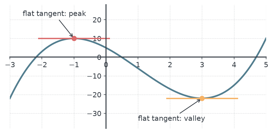
At a smooth peak or valley the graph momentarily stops rising or falling, the tangent is horizontal, so its slope \(f'(x)\) is zero.
The First-Order Condition
A point \(x^*\) with \(f'(x^*) = 0\) is called a stationary point (or critical point).
\[f'(x^*) = 0 \qquad \text{the first-order condition (FOC)}\]
- It is a necessary condition: every smooth interior extremum must be stationary
- So the FOC gives us the candidates, solve \(f'(x) = 0\) to find them all
- It is not sufficient: a flat tangent alone does not prove a peak or a valley
- Second step (next section) sorts the candidates into maxima, minima and neither
Finding the Candidates
Take \(f(x) = x^3 - 3x^2 - 9x + 5\). Where are its stationary points?
- Differentiate: \(f'(x) = 3x^2 - 6x - 9\)
- Factor: \(f'(x) = 3(x^2 - 2x - 3) = 3(x - 3)(x + 1)\)
- Set to zero: \(3(x - 3)(x + 1) = 0 \;\Rightarrow\; x = -1 \ \text{ or } \ x = 3\)
- Two candidates: \(x = -1\) and \(x = 3\), but which is a peak, which a valley?
. . .
Always factor \(f'(x)\) if you can, the stationary points are just its roots, and a factored form hands them to you directly.
Your Turn: Find the Stationary Points
NoteQuestion
Where are the stationary points of \(\;f(x) = x^3 - 12x\;\)? Shout all of them.
. . .
\[f'(x) = 3x^2 - 12 = 3(x^2 - 4) = 3(x - 2)(x + 2) = 0 \quad \Rightarrow \quad x = 2 \ \text{ or } \ x = -2\]
. . .
WarningCommon Mistake
Solving \(x^2 = 4\) as “\(x = 2\)” loses half the candidates. A square root has two signs; keep them both until the second-order test sorts them.
Marginal Revenue Meets Marginal Cost
Session 4 promised: the best output is where marginal revenue meets marginal cost. Here is why.
Profit is revenue minus cost: \(\;\pi(q) = R(q) - C(q)\).
. . .
The first-order condition \(\pi'(q) = 0\) becomes:
\[\pi'(q) = R'(q) - C'(q) = 0 \quad \Longleftrightarrow \quad R'(q) = C'(q)\]
. . .
- In words: keep producing while the next unit earns more than it costs
- Stop where the extra revenue exactly equals the extra cost, \(R' = C'\)
- The abstract “\(f'(x) = 0\)” is the business rule “marginal revenue = marginal cost”
Your Turn: Where Do They Meet?
NoteQuestion
Marginal revenue is \(R'(q) = 80 - 2q\), marginal cost is \(C'(q) = 20 + q\). At which output is profit maximal? Shout the number.
. . .
\[80 - 2q = 20 + q \quad \Rightarrow \quad 60 = 3q \quad \Rightarrow \quad q = 20\]
. . .
Below \(20\) the next unit earns more than it costs, above \(20\) it costs more than it earns: the gap between revenue and cost is widest at \(q = 20\).
Your Turn: Is a Flat Tangent Enough?
NoteQuestion
A function satisfies \(f'(2) = 0\). Does that alone tell you \(x = 2\) is a maximum or a minimum?
. . .
- No, \(f'(2) = 0\) only makes \(x = 2\) a candidate
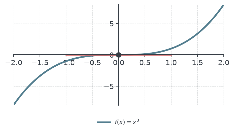
- The tangent is flat at peaks, at valleys, and at saddle points like \(f(x) = x^3\) at \(0\)
- The FOC narrows the search; deciding the type needs a second test, coming up next
Classifying Candidates: the Second-Order Condition
Peak or Valley? The Second Derivative Decides
At a stationary point \(x^*\), curvature settles the question, Session 4’s \(f''\) returns:
- \(f''(x^*) > 0\): graph is convex (bends upward), the valley of a bowl → local minimum
- \(f''(x^*) < 0\): graph is concave (bends downward), the top of a hill → local maximum
- \(f''(x^*) = 0\): the test is inconclusive, could be either, or neither
- The chord picture, made into a test: convex holds water, concave spills it
The Recipe in Four Steps
Every optimisation problem in this tutorial runs through the same four steps:
- Differentiate: compute \(f'(x)\)
- Solve \(f'(x) = 0\): the stationary points are the candidates (FOC)
- Differentiate again and evaluate \(f''\) at each candidate
- Classify: \(f'' > 0\) minimum, \(f'' < 0\) maximum, \(f'' = 0\) undecided (SOC)
. . .
Say the goal out loud first, maximise or minimise, so you know which sign of \(f''\) you are hoping for.
Classifying Our Candidates
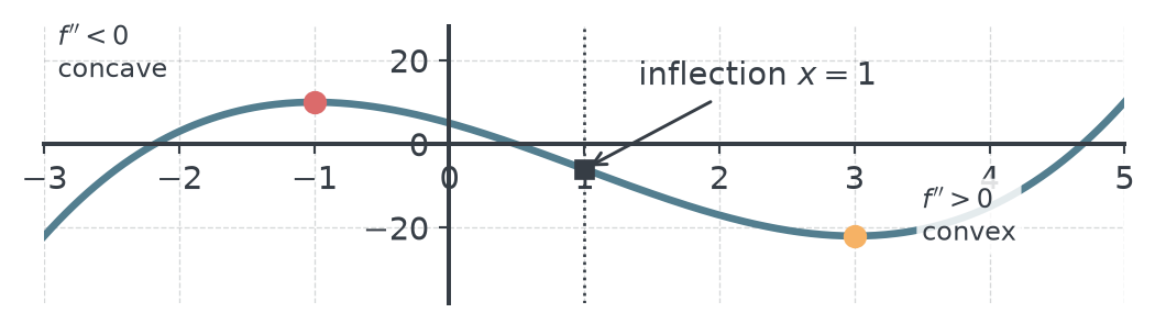
- \(f''(x) = 6x - 6\). At \(x = -1\): \(f''(-1) = -12 < 0\) → local maximum, value \(f(-1) = 10\)
- At \(x = 3\): \(f''(3) = 12 > 0\) → local minimum, value \(f(3) = -22\)
- Where \(f'' = 0\), at \(x = 1\), the bend switches: an inflection point \((1, -6)\)
Your Turn: Classify the Candidates
NoteQuestion
Back to \(f(x) = x^3 - 12x\) with stationary points \(x = 2\) and \(x = -2\). Which is which?
| (a) Maximum at \(2\), minimum at \(-2\) | (b) Minimum at \(2\), maximum at \(-2\) |
| (c) Both are minima | (d) The test is inconclusive |
. . .
(b): \(f''(x) = 6x\), so \(f''(2) = 12 > 0\) (valley) and \(f''(-2) = -12 < 0\) (peak).
. . .
Values: \(f(2) = 8 - 24 = -16\) and \(f(-2) = -8 + 24 = 16\), a local minimum of \(-16\) and a local maximum of \(16\).
When the Test Is Silent: \(f'' = 0\)
. . .
For \(f(x) = x^3\): \(f'(0) = 0\) and \(f''(0) = 0\). The tangent is flat, yet the graph keeps rising, a saddle point, neither peak nor valley.
The FOC Is Never the Whole Story
WarningCommon Mistake
Declaring “\(f'(x^*) = 0\), therefore it is a maximum”. A stationary point is only a candidate. Always check the second-order condition (or watch how \(f'\) changes sign across \(x^*\)) before naming it a max or a min.
. . .
- Alternative, the first-derivative test: if \(f'\) goes \(+ \to -\) at \(x^*\), it is a maximum; \(- \to +\), a minimum
- If \(f'\) keeps its sign across \(x^*\) (as for \(x^3\)), it is neither
- The first-derivative test always works, handy exactly when \(f'' = 0\) falls silent
The First-Derivative Test as a Table
For \(f(x) = x^3 - 3x^2 - 9x + 5\), \(f'(x) = 3(x - 3)(x + 1)\). One test point per interval:
| Interval | \(x < -1\) | \(-1 < x < 3\) | \(x > 3\) |
|---|---|---|---|
| test point | \(x = -2\) | \(x = 0\) | \(x = 4\) |
| \(f'(x)\) | \(3 \cdot (-5) \cdot (-1) = 15\) | \(3 \cdot (-3) \cdot 1 = -9\) | \(3 \cdot 1 \cdot 5 = 15\) |
| sign | \(+\) | \(-\) | \(+\) |
. . .
- At \(x = -1\) the sign flips \(+ \to -\): rising, then falling, a maximum
- At \(x = 3\) it flips \(- \to +\): falling, then rising, a minimum
- Same verdict as \(f''\), and it also works when \(f'' = 0\)
Your Turn: Max or Min?
NoteQuestion
At a stationary point \(x^*\) of a cost function, you compute \(f''(x^*) = 8 > 0\). Is \(x^*\) a local maximum or a local minimum?
. . .
- \(f''(x^*) > 0\) means the graph is convex there, a valley
- So \(x^*\) is a local minimum, exactly what you want when minimising cost
- Mnemonic: positive second derivative → holds water → minimum
Local vs Global & Boundaries
Local Is Not Global
A local optimum is best only in its neighbourhood, a bigger peak may sit elsewhere.
- The cubic’s local min at \((3, -22)\) is a valley, but \(f\) dives far lower as \(x \to -\infty\)
- On an unbounded domain, a global optimum may not exist at all
- Extreme Value Theorem: a continuous function on a closed interval \([a, b]\) always attains both a global max and a global min
- Business is usually bounded (quantities live in \([0, \text{capacity}]\)) so globals exist
The Closed-Interval Recipe
To find the global max and min of \(f\) on \([a, b]\), compare a short list:
- Find every stationary point in \((a, b)\): solve \(f'(x) = 0\)
- Evaluate \(f\) at each of them
- Evaluate \(f\) at both endpoints, \(f(a)\) and \(f(b)\)
- The largest value is the global max; the smallest is the global min
. . .
WarningCommon Mistake
Finding stationary points but forgetting the endpoints. The global optimum often sits at a boundary, skip it and you get the wrong answer.
A Boundary Can Win
Comparing the Candidates
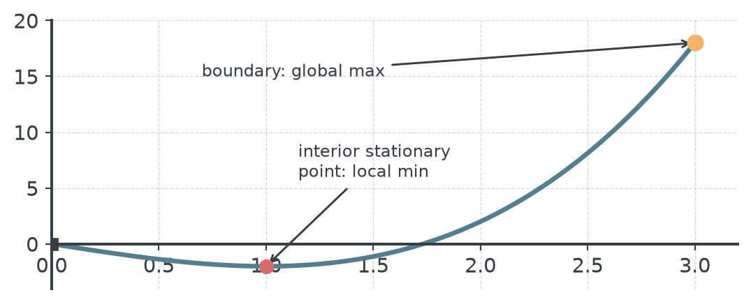
Maximise \(g(x) = x^3 - 3x\) on \([0,3]\):
| \(x\) | \(0\) (endpoint) | \(1\) (stationary) | \(3\) (endpoint) |
|---|---|---|---|
| \(g(x)\) | \(0\) | \(-2\) | \(\mathbf{18}\) |
. . .
The only interior stationary point is a minimum; the global max \(18\) sits at the boundary \(x = 3\).
Your Turn: Global on an Interval
NoteQuestion
Find the global maximum of \(\;f(x) = x^2 - 4x\;\) on \([0, 5]\). Shout the maximum value.
. . .
- Stationary point: \(f'(x) = 2x - 4 = 0 \Rightarrow x = 2\), with \(f(2) = 4 - 8 = -4\)
- Endpoints: \(f(0) = 0\) and \(f(5) = 25 - 20 = 5\)
- Compare \(\{-4, 0, 5\}\): the global maximum is \(5\), at the endpoint \(x = 5\); the stationary point is the global minimum
. . .
WarningCommon Mistake
Reporting \(-4\) because “that is where \(f' = 0\)”. An upward parabola has no interior maximum at all: on a closed interval its maximum always sits at an endpoint.
Business Domains Have Edges
Real decisions come with hard limits, and those edges are candidates:
- Quantities are non-negative: \(q \geq 0\), the edge \(q = 0\) may be optimal (produce nothing)
- Capacity caps output: \(q \leq 500\), the unconstrained optimum may lie past the limit
- When it does, the best feasible choice is the capacity boundary itself
- Model domain = mathematical domain \(\cap\) business constraints, an intersection, as in Session 2
Your Turn: The Capacity Limit
NoteQuestion
You maximise profit and the FOC gives \(q = 45\). But your plant can make at most \(40\) units, so \(q \in [0, 40]\) and profit is still rising at \(q = 40\). What is the best feasible output?
. . .
- The unconstrained optimum \(q = 45\) lies outside the feasible interval
- Profit increases all the way up to the edge, so the best feasible choice is the boundary \(q = 40\)
- Lesson: check the endpoints, a binding capacity limit is your optimum
Optimisation in Business
Setting Up a Profit Problem
We reuse Session 4’s cost function and add a revenue function:
\[C(q) = 0.5q^2 + 10q + 200 \qquad R(q) = 100q - 0.5q^2\]
- \(C\): fixed costs \(200\), rising variable costs, marginal cost \(C'(q) = q + 10\)
- \(R\): revenue peaks then falls, since selling more needs a lower price, \(R'(q) = 100 - q\)
- Profit is the gap: \(\;\pi(q) = R(q) - C(q)\)
- The plan: build \(\pi\), apply the FOC, verify with the SOC
Worked Example: Build the Profit Function
Subtract cost from revenue, term by term:
\[\pi(q) = (100q - 0.5q^2) - (0.5q^2 + 10q + 200)\]
. . .
\[\pi(q) = -q^2 + 90q - 200\]
. . .
- A downward parabola, exactly the trade-off shape from Session 3
- Differentiate: \(\;\pi'(q) = -2q + 90\)
- The fixed cost \(200\) vanishes under differentiation, it shifts profit, not the optimum
Solve and Verify
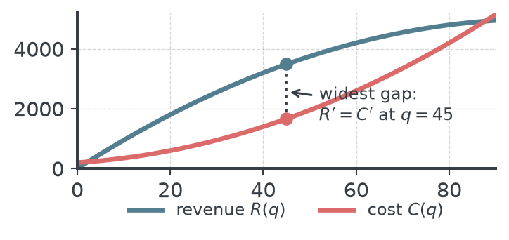
- FOC: \(\pi'(q) = -2q + 90 = 0 \;\Rightarrow\; q = 45\), and \(R'(45) = 55 = C'(45)\), marginal revenue = marginal cost
- SOC: \(\pi''(q) = -2 < 0\) → concave → a maximum, confirmed
Your Turn: Fixed Costs Rise
NoteQuestion
The rent goes up: fixed costs rise from \(200\) to \(500\), so \(C(q) = 0.5q^2 + 10q + 500\). What happens to the optimal output \(q = 45\) and to the maximum profit?
| (a) \(q\) falls, profit falls | (b) \(q\) rises, profit falls |
| (c) \(q\) unchanged, profit falls by \(300\) | (d) \(q\) unchanged, profit unchanged |
. . .
(c): \(\pi(q) = -q^2 + 90q - 500\) has the same derivative \(\pi'(q) = -2q + 90\), so the FOC still gives \(q = 45\); the constant only shifts the curve down.
. . .
Fixed costs never change the decision, only the result. That is the practical meaning of “constants differentiate to zero”.
Reading the Optimum
. . .
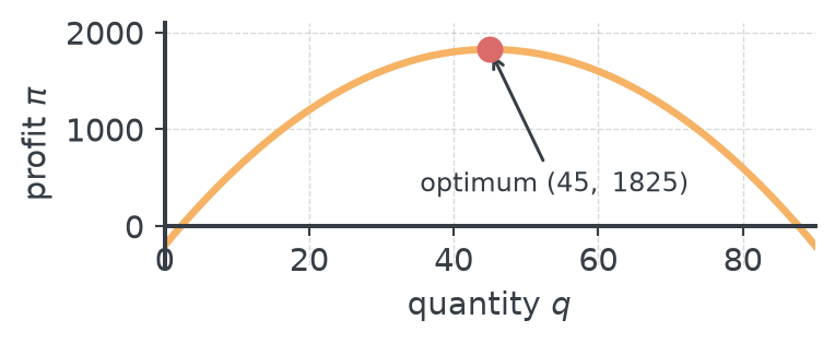
The optimal quantity is \(q = 45\), and the maximum profit is \[\pi(45) = -45^2 + 90 \cdot 45 - 200 = -2025 + 4050 - 200 = 1825,\] that is €1825, the highest point of the profit curve.
Your Turn: A Better Price
NoteQuestion
Demand improves and revenue becomes \(R(q) = 120q - 0.5q^2\), cost stays \(C(q) = 0.5q^2 + 10q + 200\). What is the new optimal output? Shout the number.
. . .
- Profit: \(\pi(q) = 120q - 0.5q^2 - 0.5q^2 - 10q - 200 = -q^2 + 110q - 200\)
- FOC: \(\pi'(q) = -2q + 110 = 0 \Rightarrow q = 55\)
- SOC: \(\pi''(q) = -2 < 0\), a maximum; and \(R'(55) = 65 = C'(55)\) ✓
Worked Example: Minimising Cost per Unit
A plant’s total cost is \(C(q) = 400 + 4q + 0.01q^2\). Which output makes the cost per unit smallest?
- Average cost: \(A(q) = \dfrac{C(q)}{q} = \dfrac{400}{q} + 4 + 0.01q\)
- Two opposing forces: the fixed cost spreads thinner (\(400/q\) falls), the variable cost per unit grows (\(0.01q\) rises)
- Rewrite for the power rule: \(A(q) = 400q^{-1} + 4 + 0.01q\)
Solve: Where Cost per Unit Bottoms Out
- FOC: \(A'(q) = -\dfrac{400}{q^2} + 0.01 = 0 \;\Rightarrow\; q^2 = 40000 \;\Rightarrow\; q = 200\)
- SOC: \(A''(q) = \dfrac{800}{q^3} > 0\) for \(q > 0\): convex, a minimum
- Value: \(A(200) = 2 + 4 + 2 = 8\), at \(200\) units each unit costs €8 on average
. . .
Notice the shape \(\frac{a}{q} + bq\): a falling term against a rising one. The next example, the most famous formula in inventory management, has exactly the same shape.
Logistics: The Economic Order Quantity
A warehouse orders a product with steady annual demand. Order too often and ordering costs pile up; order too much and holding costs pile up. Balance them.
- Annual demand \(D\), fixed cost \(K\) per order, holding cost \(h\) per unit per year, order size \(q\)
- Ordering cost: \(\frac{D}{q} \cdot K\), \(\frac{D}{q}\) orders per year, each costing \(K\)
- Holding cost: \(\frac{q}{2} \cdot h\), average stock is \(\frac{q}{2}\) (fill to \(q\), draw down to \(0\))
- Total: \(\;T(q) = \dfrac{D}{q}\,K + \dfrac{q}{2}\,h\)
Your Turn: Bigger Batches
NoteQuestion
You switch to larger orders \(q\), same annual demand \(D\). What happens to the two cost terms in \(T(q) = \frac{D}{q}K + \frac{q}{2}h\)?
| (a) Ordering cost rises, holding cost falls | (b) Ordering cost falls, holding cost rises |
| (c) Both fall | (d) Both rise |
. . .
(b): fewer orders per year (\(D/q\) shrinks), but a higher average stock (\(q/2\) grows).
. . .
Exactly this tug of war makes the total cost U-shaped, and a U has a bottom to find.
The EOQ: First-Order Condition
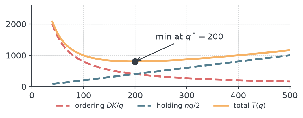
With \(D = 1000\), \(K = 80\), \(h = 4\), so \(T(q) = 80000/q + 2q\):
- FOC: \(T'(q) = -80000/q^2 + 2 = 0 \;\Rightarrow\; q^2 = 40000 \;\Rightarrow\; q^* = 200\)
The EOQ: Verify and Read
- SOC: \(T''(q) = 160000/q^3 > 0\) for all \(q > 0\) → convex → a minimum
- At \(q^* = 200\): ordering cost \(= 400\) and holding cost \(= 400\), equal, total €800
The Square-Root Formula
Solve the FOC in symbols and the classic EOQ formula drops out:
\[\frac{D K}{q^2} = \frac{h}{2} \;\Rightarrow\; q^2 = \frac{2 D K}{h} \;\Rightarrow\; \boxed{\,q^* = \sqrt{\dfrac{2 D K}{h}}\,}\]
. . .
- Check: \(\sqrt{\frac{2 \cdot 1000 \cdot 80}{4}} = \sqrt{40000} = 200\) ✓
- The optimum always balances the two costs, that is why they came out equal
- One tidy formula behind textbook inventory management, derived in four lines
Your Turn: Compute the EOQ
NoteQuestion
Annual demand \(D = 1800\) units, \(K = 25\) per order, holding cost \(h = 4\) per unit and year. What is the economic order quantity? Shout the number.
. . .
\[q^* = \sqrt{\frac{2 \cdot 1800 \cdot 25}{4}} = \sqrt{\frac{90000}{4}} = \sqrt{22500} = 150\]
. . .
Check the balance: ordering cost \(\frac{1800}{150} \cdot 25 = 300\), holding cost \(\frac{150}{2} \cdot 4 = 300\), equal, as the theory promised.
From Order Size to Order Frequency
The EOQ also fixes the rhythm of ordering:
- Orders per year: \(\dfrac{D}{q^*} = \dfrac{1800}{150} = 12\), one order a month
- Time between orders: \(\dfrac{q^*}{D}\) years \(= \dfrac{150}{1800} = \dfrac{1}{12}\) year, about \(30\) days
- In our first example (\(D = 1000\), \(q^* = 200\)): \(5\) orders a year, one every \(73\) days
. . .
The formula answers “how much”; dividing by demand answers “how often”. Both are needed for a replenishment plan.
Your Turn: Ordering Cost Doubles
NoteQuestion
A supplier doubles the fixed cost \(K\) per order. According to \(q^* = \sqrt{\frac{2DK}{h}}\), does the economic order quantity rise or fall, and by how much?
. . .
- \(q^*\) grows with \(K\) under the root, so a larger \(K\) makes \(q^*\) rise
- Doubling \(K\) multiplies \(q^*\) by \(\sqrt{2} \approx 1.41\), about a 41% larger order
- Intuition: if each order costs more, you order less often in bigger batches
Closing
Key Takeaways
- First-order condition: optima hide where \(f'(x) = 0\), solve it for the candidates
- Second-order condition: \(f''(x^*) > 0\) a minimum, \(f''(x^*) < 0\) a maximum, \(f'' = 0\) inconclusive, the FOC alone is never enough, since a flat tangent can be a saddle (\(x^3\) at \(0\))
- On a closed interval, compare stationary points and endpoints, boundaries can win
- Profit is maximal where marginal revenue = marginal cost, Session 4’s promise, delivered
- The EOQ \(q^* = \sqrt{2DK/h}\) balances ordering against holding costs
Skip order if running long: 1. Reading the Optimum plot (state \(\pi(45)=1825\) verbally on the previous slide), 2. The first-derivative-test bullets on the “FOC Is Never the Whole Story” slide, 3. Business Domains Have Edges (fold into the Your Turn capacity slide), 4. compress the R & C plot to a single sentence about the widest gap.
Until the Next Session
- Work through the Tasks: optimisation drills with worked solutions
- Check yourself with the Self-Test quiz
- Keep the Cheatsheet next to you, the FOC/SOC recipe lives on it
- Note down anything unclear, we start next session with your questions
. . .
The recipe is always the same: differentiate, set \(f' = 0\), solve, then let \(f''\) decide. Name the goal (maximise or minimise) and the sign of \(f''\) you want follows.
Preview: Session 06: Systems of Linear Equations
- Central question: solve for several unknowns at once
- From one equation to a whole system, where do the lines meet?
- Elimination and substitution, done systematically
- Gaussian elimination for bigger systems, market equilibrium, production planning
. . .
See you there, and bring your questions!
Literature & Further Reading
- These sessions cover the essentials: textbooks offer more depth and practice
- Start with Sydsæter et al. (2012) or Jacques (2015); full recommendations on the tutorial’s literature page
Jacques, Ian. 2015. Mathematics for Economics and Business. 8th ed. Always Learning. Pearson.
Sydsæter, Knut, Peter J. Hammond, and Arne Strøm. 2012. Essential Mathematics for Economic Analysis. 4th ed. Pearson.